How to Make a Poor Man’s Heat Map
Presumably you’ve got some data. Maybe it’s PITCHf/x data, maybe it’s just a bunch of data points, and you want those represented in a heat map. How do you make this happen? Well, in the spirit of leading with the lede:
Just make a scatterplot and reduce the opacity of the dots.
Yeah, it’s not elegant and it’s not truly a heat map — not algorithmically calculated like the fancy stuff Jeff makes at Baseball Heatmaps or the complex zone-grids over at FanGraphs. But, hey, for many people, it should be enough.
Let’s go ahead and make a faux heat map together!
Let’s start by ripping out some Expanded Tabled Data from Brooks Baseball and pasting that data in Excel.
For the sake of this post, we’re looking at Chris Heston’s no-hitter from June 9, 2015. Once we plop that data into Excel, we’ll want to cruise on down to the columns titled “px” and “pz.” Highlight these columns and plop in a scatterplot:
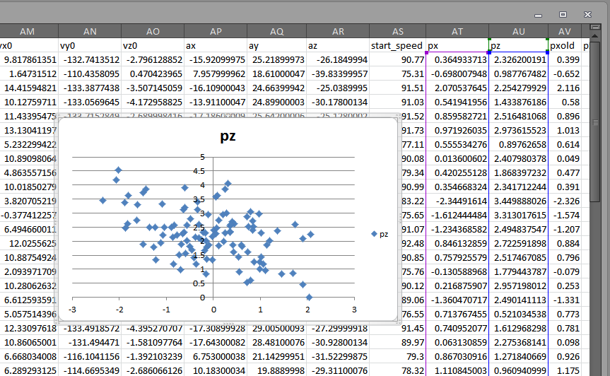
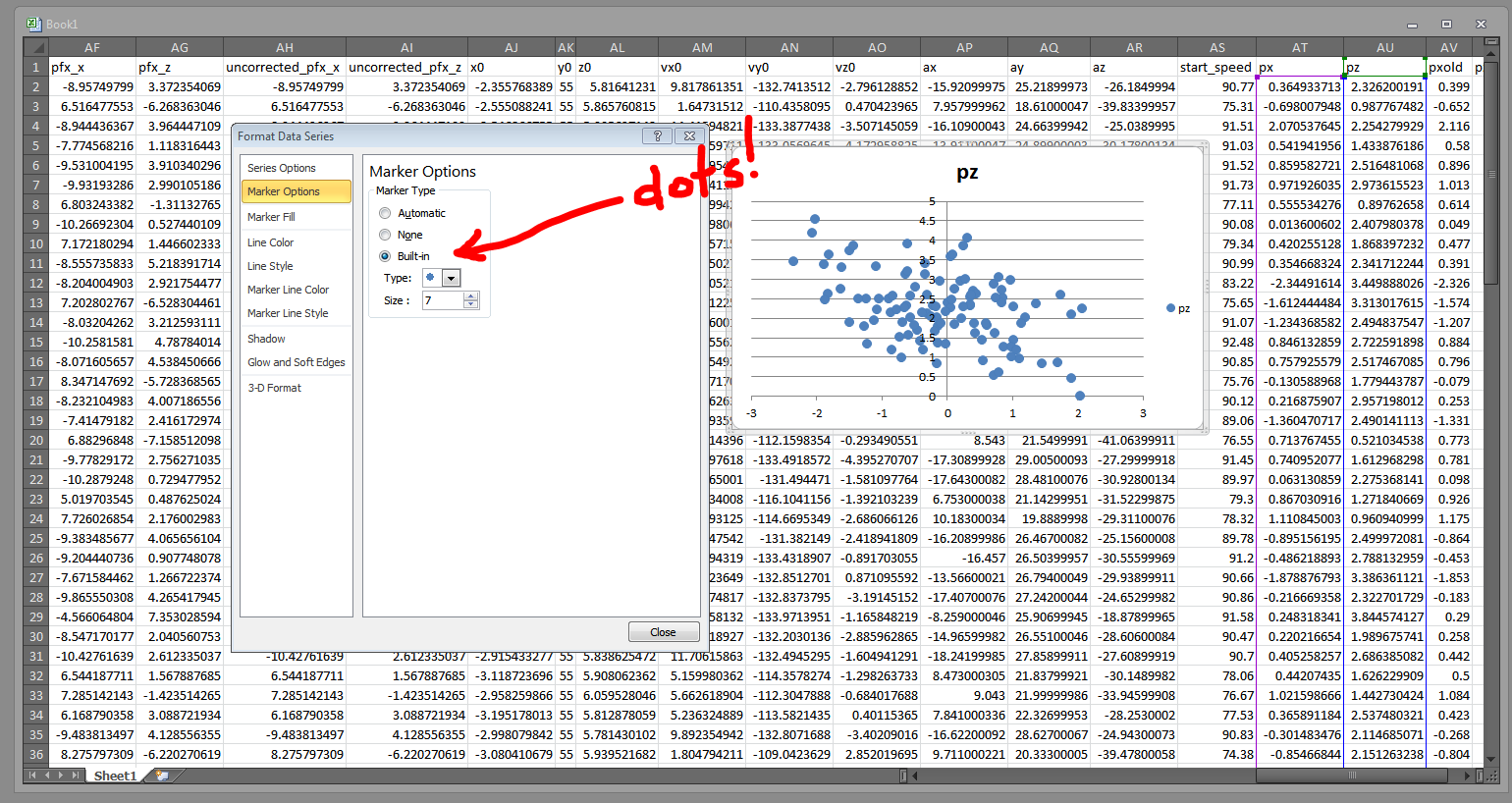
Right click on those blue diamonds and choose “Format Data Series.” Then, in the ensuing popup, browse to the “Marker Options” tab and change the markers to circles:
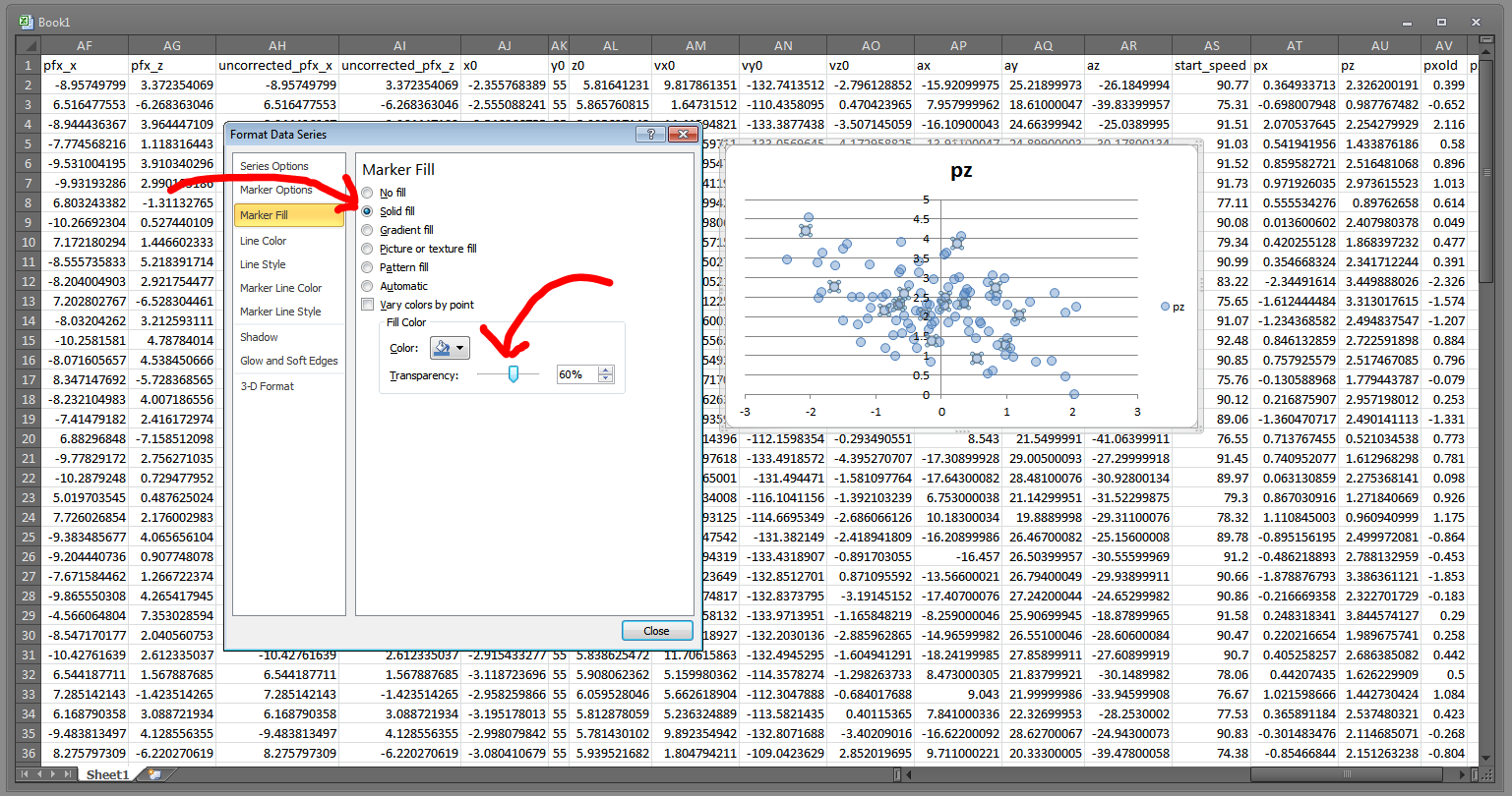
Then go to the “Marker Fill” section and choose “Solid fill.” We can then crank that transparency down:
Now we need to get rid of the pesky blue outline on each of the data points. Head to “Marker Line Color” and change that to “No line.”

So we’ve effectively got a heat map now. With a little bit of tweaking (moving the Y-axis to the left, changing the background color, making the markers bigger, and adding a quick little strikezone box — pretty much all of which you can accomplish through the Format Data Series window), we can get something like this:
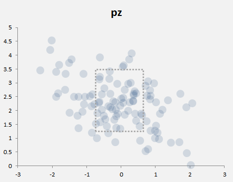
I should mention the strike zone is just a rectangle shape I inserted, and is not necessarily accurate. I set the fill to No Fill and made the border a hashed line. For specific guidance on where to put the strike zone, I suggest using Mike Fast’s article here, and then just eyeballing a shape like I did here.
Heat maps are really most useful when you have many hundreds of data points, not just one hundred. For instance, here’s a little heat map (took less then three minutes to make) that shows the correlation between HR totals and wRC+ (offensive production) for individual hitters’ seasons from 2000 through 2014. I threw in a reference line for 100 wRC+ (league average) and a linear regression trendline (in the Chart Tools > Layout section):

Here’s another one. This one took more time to cook up, but it’s 1494 records — every NFL quarterback season since 1920 who’s thrown at least 10 touchdowns. So that’s a line for every QB for every season, thus Drew Brees — for his 2009 and 2011 seasons — occupies the top two spots in the completion percentage column.
Anyway, a heatmap here really helps us see the clustering around the middle:

The transparency on the markers is at 91% (you’ll want higher transparencies for certain colors and for more data).
It’s not technically a heat map, but if you need to throw together some data to make or display a point, the built-in tools in Excel will certainly work in a pinch.