Using Vlookup for Sports Data
Modern spreadsheet programs are powerful. Compared to what our ancestors had to deal with — pen and paper spreadsheets — Excel, Google Spreadsheets, and LibreOffice / Open Office type programs are basically alien. And I mean that both in the utility and the intuitiveness of these programs. While they are incredibly useful in combing data for information, they are also full of hidden treasures — and a productivity program should never have hidden anythings.
Each of these programs has a little gem called “vlookup.” The vlookup function stands for “vertical lookup.” As we might expect, there is also a “horizontal lookup,” which is basically the same thing, but it scans columns instead of rows. The vlookup function is especially useful for when we want to combine information from across two tables. But first we need a question. Playing with data for the sake of playing with data is not super helpful — usually.
So here’s our question: Who is the most important hitter to any given team?
There are a lot of ways to approach this question, but since we want to use vlookups, let’s further this inquiry by asking: Which player has the highest wRC+ relative to the rest of his team? The weighted runs created plus (wRC+) statistic is great because it measures a players total offensive output, but it also controls for era, stadium, and league.
In order to answer this second question, we will need to know our data. We can get each individual player’s wRC+ from the FanGraphs leaderboard here. Using the Export Data button, we can get a CSV of each leaderboard page in an instant.
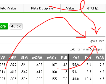
Then, we want the team data. Navigate over to the Teams tab and choose the “NP” or non-pitchers button. This gives the team-level offensive numbers without those nasty pitchers gumming up the data with their strike outs and pop outs and trickle outs.
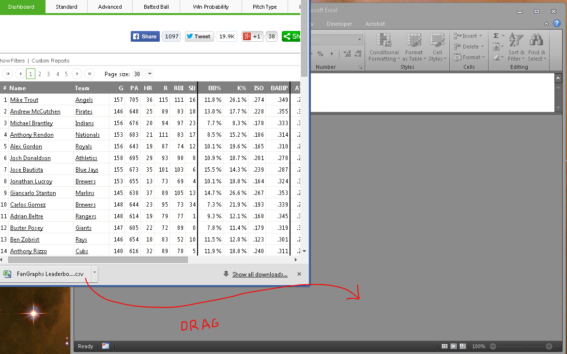
After we’ve exported both data, we can open them either by navigating to the Downloads folder and opening them with Excel, or just clicking the download icon in Chrome or Firefox or Internet Explorer if you’re stuck at work and it’s 1997. I oftentimes have multiple instances of Excel open (for my multi-monitor madness) and so I like to drag the download icon into the Excel window.
Now we have all the data we want; we just need to combine it. Enter vlookups.
To keep things neat, let’s combine our two separate workbooks. This isn’t a necessary step, but it will help our formula bars be more readable. Right click the tab of one of the worksheets (it doesn’t matter which) and choose Move or Copy…. This will open a dialogue asking where you want to move the worksheet. Using the drop down menu, choose the other workbook and click okay. This should combine the two disparate worksheets into a single workbook. (I’d also go ahead and rename them too, just for whatever’s sake.)

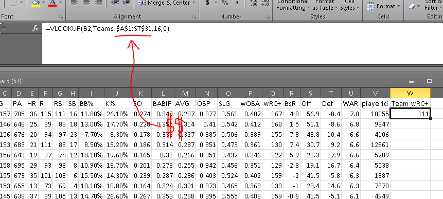
I’ve renamed my two worksheets (or tabs) as “Players” for the first set of data and “Teams” for the data we took from the teams leaderboard. On the players tab, we’ll want to add a column called “Team wRC+”. So in cell W1, I write just that, and then in cell W2 I begin to type the vlookup formula by writing =vlookup(.
The syntax for the whole formula is:
=VLOOKUP(lookup_value, table_array, col_index_num, range_lookup)
The terms:
- lookup_value: What do I want Excel to use to find something? What is the key to unlock the information door? In this case, I want Excel to find the team wRC+ by using a player’s listed wRC+, so the lookup_value needs to be B1, which is where the column “Team” is in this particular spreadsheet. (Now press comma.)
- table_array: Where is the data? Or where is the doorway for the aforementioned key? The answer to this question is the data that is in my “Teams” tab — the team totals data from our second CSV download. I’ll navigate to the Team tab, click in cell A:1 and drag until you’ve selected the whole table. Now, we don’t want this selection to move later on (because this table is not moving; it’s dead), so press F4 to add cashmoney symbols in front of your cell references. (Now press comma.)
- col_index_num: In which column will Excel find the desired data? Or where in the room is the prize? For this, we need to find which column the team wRC+ is listed in. That’s column P, which is the 16th column in our table_array (because we count every column, including the first). So here, we’ll write 16. (Now press comma.)
- range_lookup: Do we want Excel to find an exact match for the lookup_value? OF COURSE. DON’T BE SO FREAKIN’ LAZY, EXCEL. YOU’RE A ROBOT, YOU DON’T GET TIRED. Type a 0 (zero) or FALSE in here. (Now close the parenthesis and hit enter.)
Look at that! If all has gone according to plan, you should have a number populating that W2 cell (probably a “111” if Mike Trout is at the top of your list and you’re using the 2014 season data). If there is a problem and we’re getting an error message, we can always find out where that particular error is occurring by using the Evaluate Formula function (Formulas > Evaluate Formula).
Your formula, en totale, should look something like this:
Now we need to apply that formula to all the cells in the column. We can drag that bottom right corner of that “111” cell, or copy and then paste on the empty cells, or whatever the hell we want.
If all goes well, you should get a few #N/As. These mean that something went wrong in the formula. Let’s use the Evaluate Formula button (Formulas > Evaluate Formula) to find out what went wrong. If you’re using the same data as me, go to the first #N/A, which should be Chase Headley at W34.
The Evaluate Formula pop up window will then walk us through the steps of the formula and we can see the point at which it all goes terribly wrong. Clicking “Evaluate” one time shows us this:
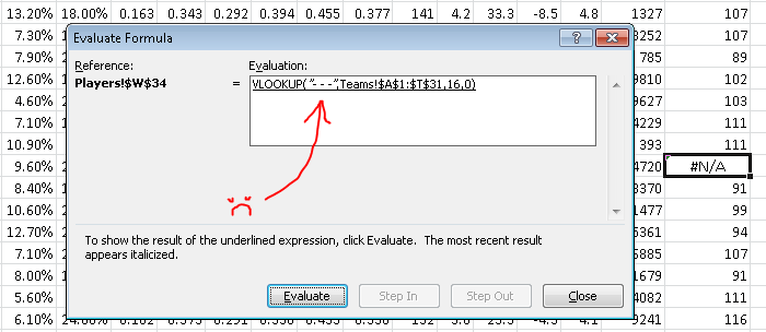
The problem here is that the formula is looking for a team named “- – -” in the Teams tab. That’s because the Padres traded Headly to the Yankees in 2014, so he has two teams on record. There’s a variety of ways to work around this (the most easy method being: check the box marked “Split Teams” on the FanGraphs leaderboard), but I just wanted to should have Evaluate Formula can be useful.
Anyway, to finish out our question (“Which hitters meant the most to their teams?”), we need some more calculations. For the ease of viewing, let’s add another column to this data. (Normally, I’d just thrust these additional calculations into the formula I’ve already got going, but that has the downside of looking complex and hiding additional errors.)
In order to get a Team+ stat (that’s the name we’ll use for our wRC+ applied to the team level), we’ll need to find the players’ differences from their team’s wRC+ and index them, the way wRC+ does. The formula for that would be something like:

Applying that Mike Trout’s 167 wRC+ and the Angels’ 111 wRC+, the formula would look like:

Putting that into Excel, we’ll get something along the lines of this:
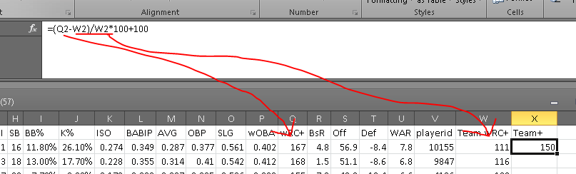
Where Q2 is the wRC+ column (Q) and Mike Trout Row (2), and W2 is the Team wRC+ column (W) and the Mike Trout row (2). For the 2014 data, this should result in Mike Trout having a 150 Team+ or thereabouts.
After applying the formula to the remaining players, we get a top five Team Most Valuable Hitters of:
| Name | Team | PA | wRC+ | Team wRC+ | Team+ |
|---|---|---|---|---|---|
| Jose Abreu | White Sox | 622 | 165 | 97 | 170 |
| Anthony Rizzo | Cubs | 616 | 153 | 93 | 165 |
| Giancarlo Stanton | Marlins | 638 | 159 | 99 | 161 |
| Adrian Beltre | Rangers | 614 | 141 | 89 | 158 |
| Seth Smith | Padres | 521 | 133 | 88 | 151 |
Well done, Mr. Rookie! Jose Abreu may not have had as strong a season as Andrew McCutchen — the league’s top hitter — but nobody meant more to his lineup than Abreu, according to the measures we’re using here.
I hope this instruction was helpful. Let me know if you have additional questions.
What is the advantage of VLOOKUP over Index(Match())?
I’m curious about this as well. I stopped using VLookup in favor of Index and Match a couple years ago.
Two advantages I can think of:
1) Vlookup is easier to understand and more widely used.
2) Vlookup allows for non-exact matches (by entering true in the last argument). This is extremely useful when you want to put values into various categories or buckets based on what ranges they fall in.
That being said, Index Match is better overall as it has much more flexibility than vlookup.
Match allows non-exact as well, and I switched to Index because it seemed easier to use for me.
So, I still do not see a technichal advantage to Vlookup, but people may use it based on familiarity and personal preference.
If you’re sharing spreadsheets in your work (like I often do), the Vlookup can be a lot easier to read for simple lookups, so it can make things simpler for a later user.
But otherwise, I agree the Index/Match combo lets you do a lot more.
Yes, and I totally agree that INDEX-MATCH is far more powerful too. I use VLOOKUP more, though, simply because it’s one formula instead of two.
Whenever I am search two dimensions of data (such as a matrix), I obviously have to use INDEX-MATCH, but since I am usually just looking up data stored in a traditional table, VLOOKUP does the job well enough. As the commentor tz says below, VLOOKUP is also just easier to read. And sometimes I have to audit a particularly big and nasty, multi-layered IF formula, and having VLOOKUPs keeps things simple.
But if Lt. Gen. Excel matched his troops onto my lawn and said it’s INDEX-MATCH or die!, I’d say okay, whutevz.
Nice work Bradley! I remember when I first figured out how VLOOKUP worked. It was great, it allowed me to do much more than before.
Have you ever tried the INDEX-MATCH combination? Since I learned about it and figured it out, I’ve never gone back to VLOOKUP. It allows you to do everything that VLOOKUP does (I think), and more! Like you can easily match on a number of columns at once (i.e. the player ID AND year have to match). I find the syntax easier to remember too.
The syntax is basically INDEX(, MATCH(&,&,0), 0). Something like that. If that’s even readable. I can’t even remember what the zeroes are for at the end, as I’ve never changed them.
Anyway it’s another option to consider if you feel like it some time. I prefer it, but you may not of course!
Wow, I had put some text inside angled brackets in the syntax, which got stripped away in the comment. Anyway you can look it up, or I’ll try one more time without the brackets:
INDEX(column that you want to grab data from, MATCH(cell1 that needs to match&cell2 that needs to match,column1 to find match&column2 to find match,0), 0).
See my response above. As for the syntax, I won’t argue that VLOOKUP is weird in that regard. I’m so accustomed to it now, though, that it doesn’t bother me.
Because of this column, I have just taught myself INDEX MATCH this morning. It was a good morning.
There’s a part of VLOOKUP that drives me nuts: the hardcoded column index constant. Any perturbation (e.g. insert or delete) of the columns prior to your index number causes the column index to no longer be valid. I’m surprised that Excel doesn’t let you specify the column letter/name for the column index.
Would the INDEX-MATCH combo work around that?
You can use the COLUMN formula along with Structured References (Table References) to return a somewhat variable column argument into the VLOOKUP formula. You can get a glimpse at step #22 on this post. http://www.smartfantasybaseball.com/2013/03/create-your-own-fantasy-baseball-rankings-part-3-vlookupseexcel-tables-excel-named-ranges/
I’ll be making a vlookup video soon (using both baseball and football data), and I will cover a solution for that. In short: Use Table formats and names. That way you can change the content of the tables and it’s all gravy.
EDIT: Or take a gander at Tanner’s link up there.
Reporting back, the INDEX-MATCH combo does deal with column insertions well. Using tables, despite the great information from Tanner via the link, was sub-optimal for me because I have multiple instances of columns with the same name. I did not want to go through any machinations rename them or hide part of their name.
Thanks for the assists gentlemen!