How to Get the Most Out of “Format as a Table”

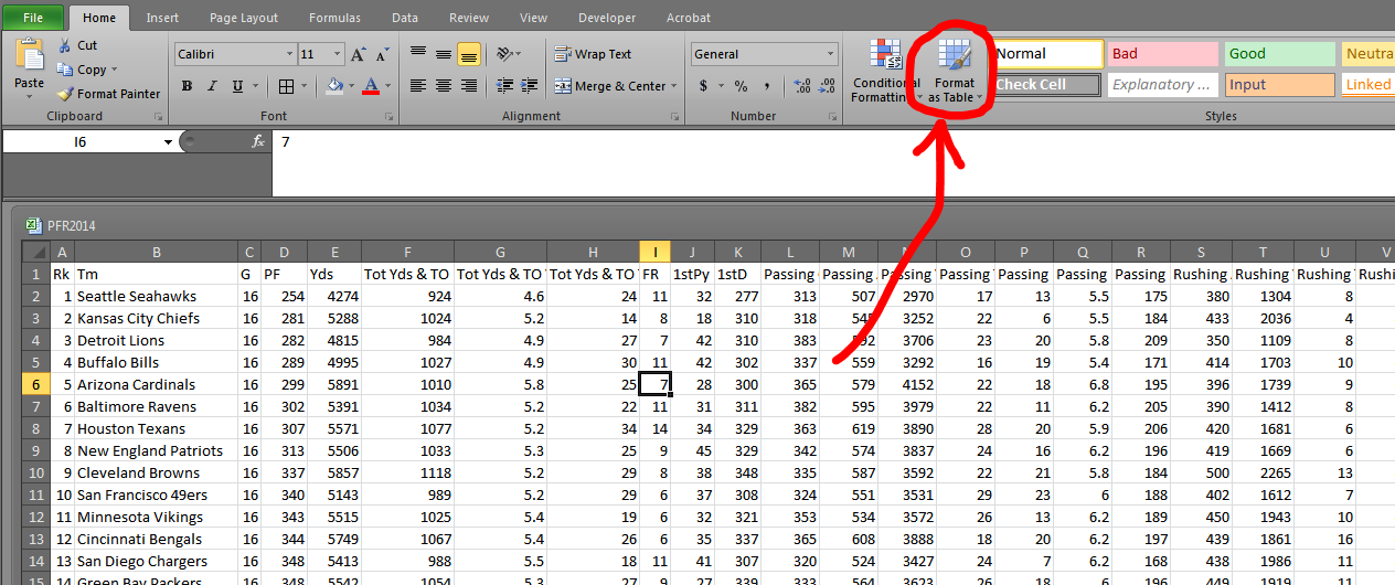
One of the Excel features that I feel too many people ignore is the “Format as a Table” tool. Let’s say we’ve got this data, 2014 team defense data from Pro-Football-Reference.com. I’ve cleaned it up a little — gotten rid of the totals at the bottom and consolidated the headers into one row — but it should still be a fairly recognizable table.

File -> PFR2014.csv

The process of formatting data as a table is really stupidly simple. Click anywhere within the table’s data (so anywhere from A1 to Z33). Now choose “Format as a Table” from the Home tab:

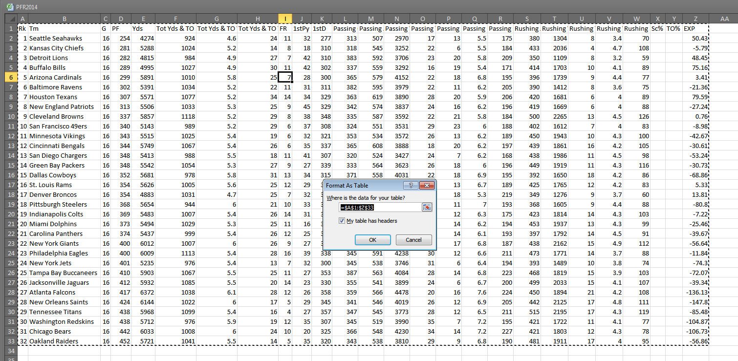
I am going to select the third from the top red design because red is the greatest color. When I do pick that design, I get a popup and a blinking border around my data:

Presto magnifico, I have a table!

“But Bradley, you had a table all along.”

Shut up, and yes, I did — but this one is better. Lemme show you why.

The first thing I like to do is enable “Wrap Text” on the header row (select the top row, then Home > Wrap Text). It allows me to see the whole table much better. (This is a simple operation, but if you’re confused, Professor Google should have a plethora of resources on the matter.)

The second thing I like to do is rename this table — especially if I’m going to do work with multiple tables. To rename the table, head to Formulas > Name Manager. The name manager popup window should have only one table in it — Table1. Double click that line, and a subsequent pop up will enable us to edit the name:

Once you choose a name, click OK then Close. Now when we select all the data in the table, it will highlight the name “Defense” in a names drop-down menu:

Of course, we can name a table without it being formatted through the “Format as Table” function. But what’s nice about the “Format” table is that if I add a row or a column, the named table “Defense” automatically expands. Let’s try this out.

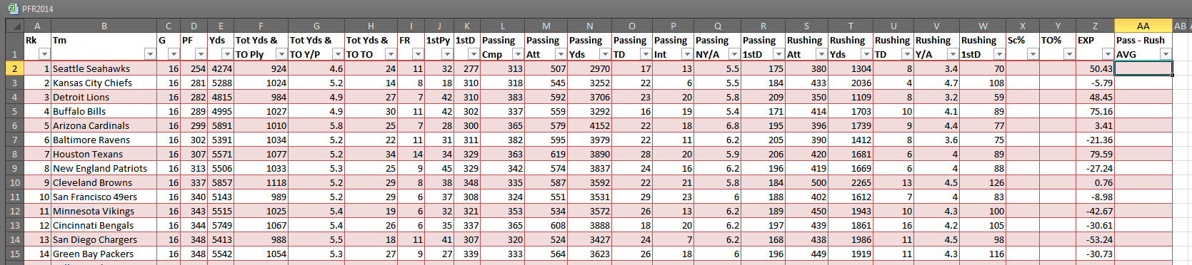
Go to cell AA1 and type “Pass – Rush AVG” (we’re going to create a new column). Excel will automatically create and format a new column, like this:

Now, I’m going to type a new formula into it:

=[Passing NY/A]-[Rushing Y/A]

Whoa! That’s not a normal Excel formula! That’s right. It’s a table formula. Now that we have a named table, we can use the column names to complete formulas within (and without) the table. More on that in a second.

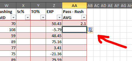
Depending on your settings, the formula may have automatically filled to the bottom of the spreadsheet. If it didn’t, just click on the autofill icon that appeared at the bottom left corner, and choose to allow the formula to overwrite the contents of the column:

And hey, remember that strange formula we made a second ago? Let’s do something similar on a different tab. I’m going to add another sheet, Sheet2, and type into any cell:

=AVERAGE(Defense[Pass - Rush AVG])

That’s a basic =AVERAGE formula, but because of the named table “Defense” and the named column “Pass – Rush AVG,” I’m able to write the formula without using the mouse or worrying about cells moving or data changing. In fact, I can go back and change the name of that column to “Net Pass AVG” and guess what happens to my formula? It changes automatically to:

=AVERAGE(Defense[Net Pass AVG])

One of the biggest advantages to using named tables (and editing those table names) is that when formula get REALLY complicated, you can read something that’s close to English, not a collection of meaningless cell references (“Wait, was A1:D22 the running data? Or was that in F2:Y54?” as opposed to “Oh, I have Running[AVG] not Running[Data] selected. Oops!”).

Consider this formula from my Scoresheet dataset:

=IF(VLOOKUP(CONCATENATE([@firstName]," ",[@lastName]),FGDC,19,0)=0,"",VLOOKUP(CONCATENATE([@firstName]," ",[@lastName]),FGDC,19,0))

“FGDC” is data pulled from the FanGraphs Depth Charts leaderboard. I have that data on a separate tab. Here’s how the above formula would look without named sections:

=IF(VLOOKUP(CONCATENATE(Combined!G2:G1010," ",Combined!H2:H1010),'FG DC'!A2:X1141,19,0)=0,"",VLOOKUP(CONCATENATE(Combined!G2:G1010," ",Combined!H2:H1010),'FG DC'!A2:X1141,19,0))

Both formulas are unwieldy, but at least the first one is intrinsically sensible. I’m combining the column “firstName” with “lastName” and looking them up in table FGDC. If I don’t find them, then I want Excel to put nothing into the cell (i.e. print “”).

If you want to learn more about structured references, I recommend this rundown of the syntax and various uses of structured refs.

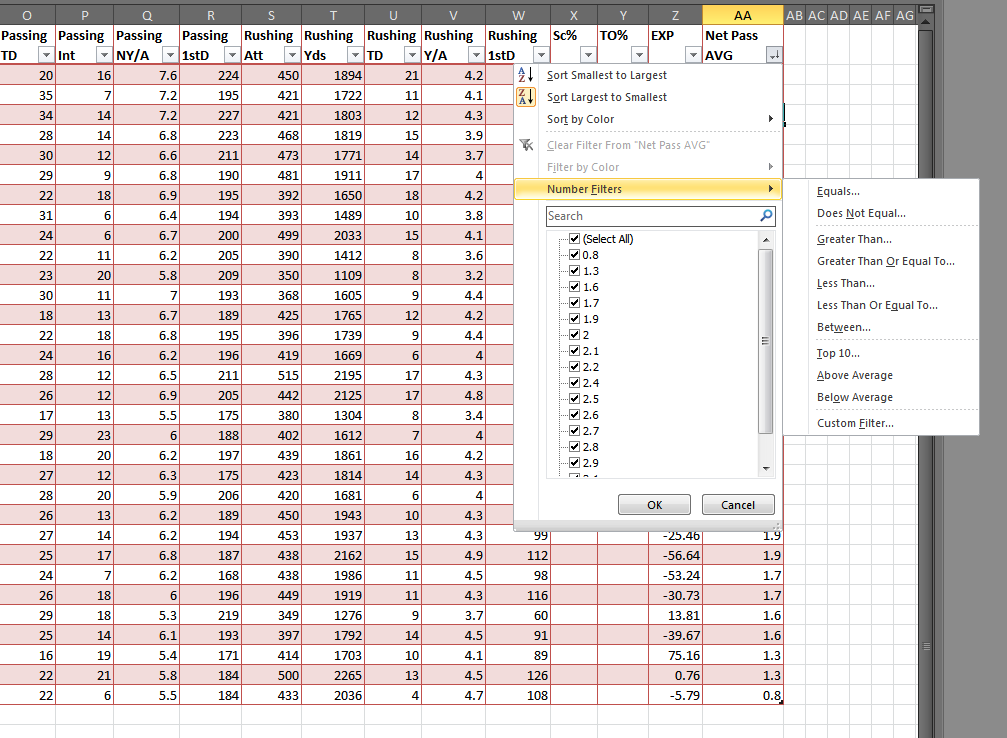
It’s also important to note a named table automatically adds filters and applies those filters even to new columns and rows.

Another small, but useful component of tables is that the jump shortcuts (e.g. CTRL+→) will jump to the end of the table, even if the row or column is empty. In other words, in the empty Sc% column, if we press CTRL+↓, the cursor will move to X33 instead of X1048576, which is where it would normally and uselessly end.

There’s a multitude of other little handy features when it comes to structured tables, like being able to neatly and easily select whole columns of data without also selecting the header and the empty cells beneath the data. But for now, I hope this is enough to get the Excel newbie started with exploring this surprisingly robust feature.